4 Time series

Roadmap of time series analysis:

Part 1 Random walk approach:

Data –> Stationarity? –>(ADF test) -Yes-> Plot ACF –> Autocorrelation? -Yes-> Not a random walk (No —> It is a random walk)

—Not Stationarity–> Apply transformations/ differencing (e.g., log function to stabilise its variance, first-order differencing)

Part 2 ARIMA approach:

Non-stationarity –> find the d (differenced times) –> list(p, q) (from ACF and PACF) –> ARIMA (p, d, q) –> AIC optimisation –> Residual analysis (Q-Q plot, Uncorrelated)–> Forecasting

4.1 Time series analysis fundamentals

Defination: A time series is a collection of data points ordered in time. Typically, these data points are spaced at consistent intervals, such as hourly, monthly, or yearly.

Decomposition: Time series decomposition is a process by which we separate a time series into its components: trend, seasonality, and residuals.

• The trend represents the slow-moving changes in a time series. It is responsible for making the series gradually increase or decrease over time.

• The seasonality component represents the seasonal pattern in the series. The cycles occur repeatedly over a fixed period of time.

• The residuals represent the behavior that cannot be explained by the trend and seasonality components. They correspond to random errors, also termed white noise.

4.1.1 Random walk

A random walk is a process in which there is an equal chance of going up or down by a random number.

In other words, a random walk is a series whose first difference is stationary and uncorrelated.

This means that the process moves completely at random.

Note: Because a random process takes random steps into the future, we cannot use statistical or deep learning techniques to fit such a process:

there is nothing to learn from randomness and it cannot be predicted. Instead, we must rely on naive forecasting methods (df.shift()).

4.1.2 Stationarity

A stationary time series is one whose statistical properties do not change over time.

In other words, it has a constant mean, variance, and autocorrelation, and these properties are independent of time.

Some models assume stationarity: The moving average model (MA), autoregressive model (AR), and autoregressive moving average model(ARMA).

Augmented Dickey-Fuller (ADF) test

The augmented Dickey-Fuller (ADF) test helps us determine if a time series is stationary by testing for the presence of a unit root.

If a unit root is present, the time series is not stationary.

The null hypothesis states that a unit root is present, meaning that our time series is not stationary.

You can download the sample data from here.

import pandas as pd
import numpy as np

# load the sample data
df_data = pd.read_csv('ts_sample_data.csv', index_col=0)

df_data

	date	data
0	2021-01-01	0.71
1	2021-01-02	0.63
2	2021-01-03	0.85
3	2021-01-04	0.44
4	2021-01-05	0.61
...	...	...
79	2021-03-21	9.99
80	2021-03-22	16.20
81	2021-03-23	14.67
82	2021-03-24	16.02
83	2021-03-25	11.61

84 rows × 2 columns

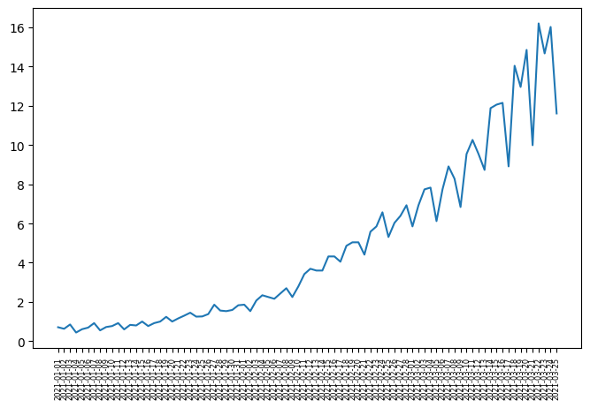
# plot the time series data
import matplotlib.pyplot as plt
plt.figure(figsize=(8, 5))
plt.plot(df_data.date.values, df_data.data.values)
plt.xticks(fontsize=6, rotation=90)  # Adjust font size and rotation angle
plt.show()

from statsmodels.tsa.stattools import adfuller

# ADF test
ADF_result = adfuller(df_data.data)
print(f'ADF Statistic: {ADF_result[0]}')
print(f'p-value: {ADF_result[1]}')

ADF Statistic: 2.7420165734574753
p-value: 1.0

Interpretation: The p-value greater than 0.05, we cannot reject the nullhypothesis stating that our time series is not stationary.

4.1.3 Differencing

One-Step differencing

diff_data1 = np.diff(df_data.data, n=1) # n=1 is one-step

print(df_data.data.values)

[ 0.71      0.63      0.85      0.44      0.61      0.69      0.92
  0.55      0.72      0.77      0.92      0.6       0.83      0.8
  1.        0.77      0.92      1.        1.24      1.        1.16
  1.3       1.45      1.25      1.26      1.38      1.86      1.56
  1.53      1.59      1.83      1.86      1.53      2.07      2.34
  2.25      2.16      2.43      2.7       2.25      2.79      3.42
  3.69      3.6       3.6       4.32      4.32      4.05      4.86
  5.04      5.04      4.41      5.58      5.85      6.57      5.31
  6.03      6.39      6.93      5.85      6.93      7.74      7.83
  6.12      7.74      8.91      8.28      6.84      9.54     10.26
  9.54      8.729999 11.88     12.06     12.15      8.91     14.04
 12.96     14.85      9.99     16.2      14.67     16.02     11.61    ]

print(diff_data1) # -0.08 = 0.63(y_t) - 0.71(y_t-1)

[-0.08      0.22     -0.41      0.17      0.08      0.23     -0.37
  0.17      0.05      0.15     -0.32      0.23     -0.03      0.2
 -0.23      0.15      0.08      0.24     -0.24      0.16      0.14
  0.15     -0.2       0.01      0.12      0.48     -0.3      -0.03
  0.06      0.24      0.03     -0.33      0.54      0.27     -0.09
 -0.09      0.27      0.27     -0.45      0.54      0.63      0.27
 -0.09      0.        0.72      0.       -0.27      0.81      0.18
  0.       -0.63      1.17      0.27      0.72     -1.26      0.72
  0.36      0.54     -1.08      1.08      0.81      0.09     -1.71
  1.62      1.17     -0.63     -1.44      2.7       0.72     -0.72
 -0.810001  3.150001  0.18      0.09     -3.24      5.13     -1.08
  1.89     -4.86      6.21     -1.53      1.35     -4.41    ]

# ADF test for diff data
ADF_result = adfuller(diff_data1)
print(f'ADF Statistic: {ADF_result[0]}')
print(f'p-value: {ADF_result[1]}')

ADF Statistic: -0.4074097636380318
p-value: 0.9088542416911329

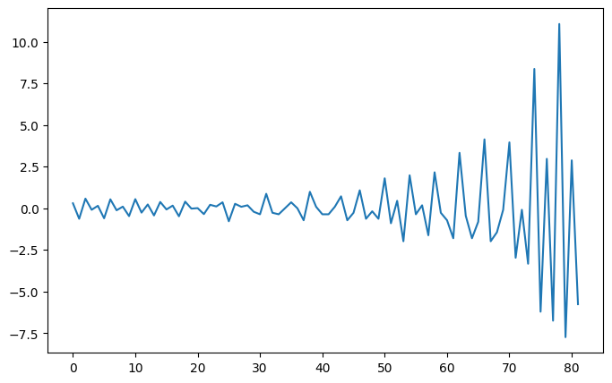
Two-Step differencing as p > 0.05 after one-step

diff_data2 = np.diff(df_data.data, n=2) # n=2 is two-step

print(diff_data1) # one-step sereis

[-0.08      0.22     -0.41      0.17      0.08      0.23     -0.37
  0.17      0.05      0.15     -0.32      0.23     -0.03      0.2
 -0.23      0.15      0.08      0.24     -0.24      0.16      0.14
  0.15     -0.2       0.01      0.12      0.48     -0.3      -0.03
  0.06      0.24      0.03     -0.33      0.54      0.27     -0.09
 -0.09      0.27      0.27     -0.45      0.54      0.63      0.27
 -0.09      0.        0.72      0.       -0.27      0.81      0.18
  0.       -0.63      1.17      0.27      0.72     -1.26      0.72
  0.36      0.54     -1.08      1.08      0.81      0.09     -1.71
  1.62      1.17     -0.63     -1.44      2.7       0.72     -0.72
 -0.810001  3.150001  0.18      0.09     -3.24      5.13     -1.08
  1.89     -4.86      6.21     -1.53      1.35     -4.41    ]

print(np.array([f"{_:.2f}" for _ in diff_data2])) # 0.30 = 0.22(y_k) - (-0.08)(y_k-1): k is one-step sereis index

['0.30' '-0.63' '0.58' '-0.09' '0.15' '-0.60' '0.54' '-0.12' '0.10'
 '-0.47' '0.55' '-0.26' '0.23' '-0.43' '0.38' '-0.07' '0.16' '-0.48'
 '0.40' '-0.02' '0.01' '-0.35' '0.21' '0.11' '0.36' '-0.78' '0.27' '0.09'
 '0.18' '-0.21' '-0.36' '0.87' '-0.27' '-0.36' '0.00' '0.36' '0.00'
 '-0.72' '0.99' '0.09' '-0.36' '-0.36' '0.09' '0.72' '-0.72' '-0.27'
 '1.08' '-0.63' '-0.18' '-0.63' '1.80' '-0.90' '0.45' '-1.98' '1.98'
 '-0.36' '0.18' '-1.62' '2.16' '-0.27' '-0.72' '-1.80' '3.33' '-0.45'
 '-1.80' '-0.81' '4.14' '-1.98' '-1.44' '-0.09' '3.96' '-2.97' '-0.09'
 '-3.33' '8.37' '-6.21' '2.97' '-6.75' '11.07' '-7.74' '2.88' '-5.76']

# ADF test for diff data
ADF_result = adfuller(diff_data2)
print(f'ADF Statistic: {ADF_result[0]}')
print(f'p-value: {ADF_result[1]}')

ADF Statistic: -3.5851628747931596
p-value: 0.006051099869603575

Interpretation: Two step time series is stationanry as p < 0.05.

# plot the two step time series data
import matplotlib.pyplot as plt
plt.figure(figsize=(8, 5))
plt.plot(diff_data2)
plt.show()

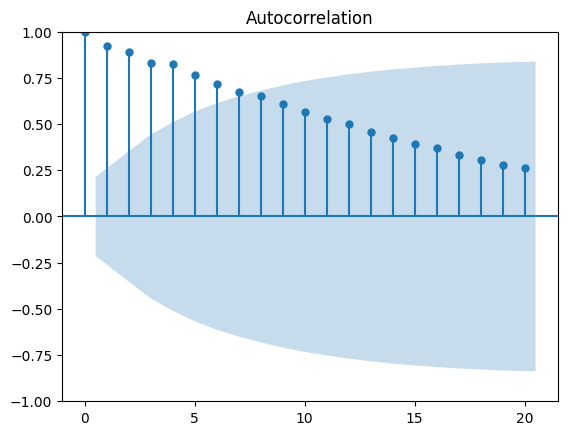
4.1.4 The autocorrelation function (ACF)

The autocorrelation function (ACF) measures the linear relationship between lagged values of a time series.

In other words, it measures the correlation (covariance) of the time series with itself.

\(\text{Cov}(x_t, x_{t-k}) = \frac{1}{N} \sum_{t=k+1}^{N} (x_t - \mu)(x_{t-k} - \mu)\)

• \(k\) is the lag;

• \(x_t\) is the value at time \(t\) ;

• \(x_{t-k}\) is the value at time \(t-k\) ;

• \(\mu\) is the mean of the time series ;

• \(N\) is the number of observations.

from statsmodels.graphics.tsaplots import plot_acf

# X-Axis: Displays the lag values.
# Y-Axis: Displays the autocorrelation values ranging from -1 to 1.
# Note that the shaded area represents a confidence interval. 
# If a point is within the shaded area, then it is not significantly different from 0.
# Otherwise, the autocorrelation coefficient is significant.
plot_acf(df_data.data, lags=20)
plt.show()

4.2 MA(\(q\)), AR(\(p\)),ARMA (\(p\),\(q\)) models

4.2.1 Moving average model (MA) – (\(q\))

In a moving average (MA) process, the current value depends linearly on the mean of the series, the current error term, and past error terms.

The moving average model is denoted as MA(\(q\)), where \(q\) is the order.

The general expression of an MA(\(q\)) model is:

\[ y_t = \mu + \epsilon_t + \theta_1 \epsilon_{t-1} + \theta_2 \epsilon_{t-2} + \cdots + \theta_q \epsilon_{t-q} \]

• The present (\(t\)) error term \(\epsilon_t\) , and past error terms \(\epsilon_{t-q}\) ;

• The magnitude of the impact of past errors on the present value is quantified using a coefficient denoted as \(\theta_q\) .

4.2.2 Autoregressive model (AR) – (\(p\))

An autoregressive process is a regression of a variable against itself.

In a time series, this means that the present value is linearly dependent on its past values.

The autoregressive process is denoted as AR(\(p\)), where \(p\) is the order.

The generalexpression of an AR(\(p\)) model is:

\[y_t = C + \phi_1 y_{t-1} + \phi_2 y_{t-2} + \cdots + \phi_p y_{t-p} + \epsilon_t\]

• A constant \(C\);

• The present error term \(\epsilon_t\) , which is also white noise;

• The past values of the series \(y_{t-p}\);

• The magnitude of the influence of the past values on the present value is denoted as \(\phi_p\), which represents the coefficients of the AR (\(p\)) model.

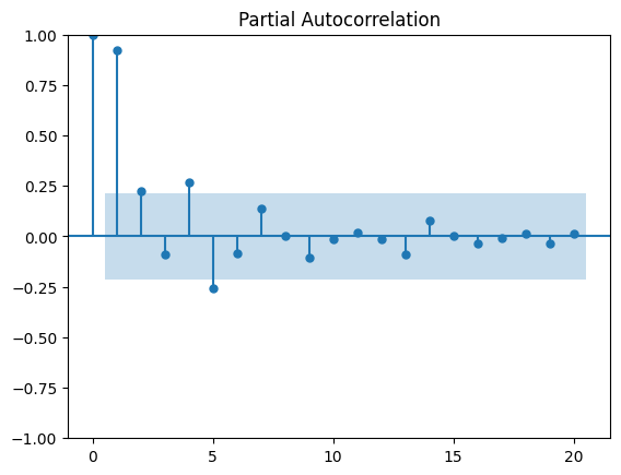
Partial autocorrelation measures the correlation between lagged values in a time series when we remove the influence of correlated lagged values in between.

It measures the direct relationship between an observation and its lag, removing the effect of the intermediate lags.

It essentially gives the partial correlation of a time series with its own lagged values, controlling for the effect of other lags.

We can plot the partial autocorrelation function to determine the order of a stationary AR(\(p\)) process.

The coefficients will be non-significant after lag \(p\).

from statsmodels.graphics.tsaplots import plot_pacf

# Plot partial autocorrelation
plot_pacf(df_data.data, lags=20)
plt.show()

4.2.3 Autoregressive moving average model (ARMA) – (\(p\), \(q\))

The autoregressive moving average process is a combination of the autoregressive process and the moving average process.

It is denoted as ARMA(\(p\),\(q\)), where \(p\) is the order of the autoregressive process, and \(q\) is the order of the moving average process.

The general equation of the ARMA(\(p\),\(q\))model is:

\[y_t = C + \phi_1 y_{t-1} + \phi_2 y_{t-2} + \cdots + \phi_p y_{t-p} + \mu + \epsilon_t + \theta_1 \epsilon_{t-1} + \theta_2 \epsilon_{t-2} + \cdots + \theta_q \epsilon_{t-q} \]

Note:

• An ARMA(\(0,q\)) process is equivalent to an MA(\(q\)) process, since the order \(p = 0\) cancels the AR(\(p\)) portion.

• An ARMA(\(p,0\)) process is equivalent to an AR(\(p\)) process, sincethe order \(q = 0\) cancels the MA(\(q\)) portion.

4.3 ARIMA – (\(p\), \(d\), \(q\))

An autoregressive integrated moving average (ARIMA) model is the combination of the AR(\(p\)) and MA(\(q\)) processes, but in terms of the differenced series.

It is denoted as ARIMA(\(p,d,q\)), where \(p\) is the order of the AR(\(p\)) process, \(d\) is the order of integration, and \(q\) is the order of the MA(\(q\)) process.

Integration is the reverse of differencing, and the order of integration \(d\) is equal to the number of times the series has been differenced to be rendered stationary.

The general equation of the ARIMA(\(p,d,q\)) process is:

\[y'_t = \Delta^d y_t\]

\[y'_t = C + \phi_1 y'_{t-1} + \dots + \phi_p y'_{t-p} + \theta_1 \epsilon'_{t-1} + \dots + \theta_q \epsilon'_{t-q} + \epsilon_t\]

Note that \(y'_t\) represents the differenced series after \(d\) times, and it may have been differenced more than once.

The Akaike information criterion (AIC) is a measure of the quality of a model in relation to other models.

It is used for model selection.

The AIC is a function of the number of parameters \(k\) in a model and the maximum value of the likelihood function \(\hat{L}\):

\[ \text{AIC} = 2k - 2 \ln(\hat{L}) \]

The lower the value of the AIC, the better the model.

Selecting according to the AIC allows us to keep a balance between the complexity of a model and its goodness of fit to the data.

SARIMAX is acomplex algrithm that allows us to consider seasonal effects, autoregressive processes, non-stationary time series, moving average processes, and exogenous variables all in asingle model.

Key parameters for ARIMA model in SRIMAX algorithm:

• endog: time series y

• order: (p, d, q)

Step1: Set optimization function for ARIMA parameter tuning using AIC

from typing import Union
from statsmodels.tsa.statespace.sarimax import SARIMAX

def optimize_ARIMA(endog: Union[pd.Series, list], order_list: list, d: int):
    results = []
    for order in order_list:
        try:
            model = SARIMAX(endog, order=(order[0], d, order[1]), simple_differencing=False).fit(disp=False)
            aic = model.aic
            results.append([order, aic])
        except Exception as e:
            # Print or log the exception if needed
            print(f"Error encountered for order {order}: {str(e)}")
            continue

    # Convert results to DataFrame and sort by AIC
    result_df = pd.DataFrame(results, columns=['(p,q)', 'AIC'])
    result_df = result_df.sort_values(by='AIC', ascending=True).reset_index(drop=True)
    return result_df

Step2: Set parameter ranges

from itertools import product
ps = range(0, 4, 1) # set p range 
qs = range(0, 4, 1) # set q range 
d = 2 # set d (this can be range as well)
order_list = list(product(ps, qs))
print(order_list)

[(0, 0), (0, 1), (0, 2), (0, 3), (1, 0), (1, 1), (1, 2), (1, 3), (2, 0), (2, 1), (2, 2), (2, 3), (3, 0), (3, 1), (3, 2), (3, 3)]

Step3: Training

# training set and testing set
train_data = df_data.data[:-4]
test_data = df_data.data[-4:]

%%time

import warnings
warnings.filterwarnings('ignore')

result_df = optimize_ARIMA(train_data, order_list, d)

CPU times: user 809 ms, sys: 2.94 s, total: 3.75 s
Wall time: 1.38 s

result_df

	(p,q)	AIC
0	(3, 3)	115.268398
1	(3, 1)	115.624980
2	(3, 2)	115.672006
3	(3, 0)	154.430628
4	(0, 3)	194.654716
5	(0, 2)	209.274500
6	(2, 3)	220.666883
7	(1, 3)	228.267671
8	(1, 2)	228.935804
9	(2, 2)	229.974748
10	(2, 1)	234.501112
11	(1, 1)	236.117282
12	(0, 1)	252.601059
13	(2, 0)	280.299907
14	(1, 0)	280.389386
15	(0, 0)	320.324435

Step4: Selecting the best p,d,q for ARIMA

model = SARIMAX(train_data, order=(3,2,3), simple_differencing=False) # Selecting the best p,d,q for ARIMA
model_fit = model.fit(disp=False) 

Step5: Residual analysis/diagnosis

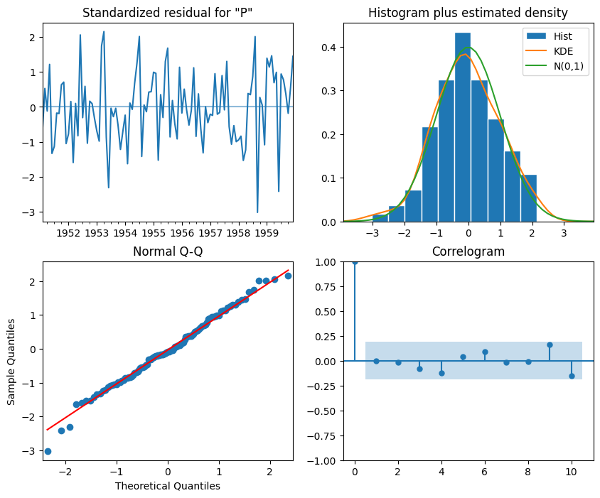
# plot_diagnostics
model_fit.plot_diagnostics(figsize=(10,8)) 
plt.show()

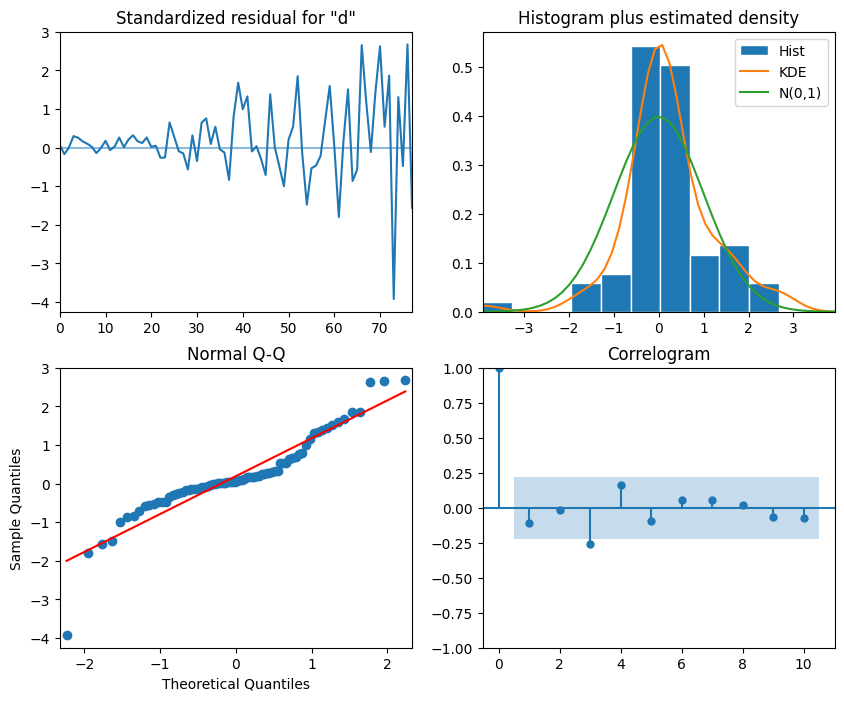
Interpretation:

• The top-left plot shows the residuals over time: While there is no trend in the residuals, the variance does not seem to be constant, which is a discrepancy in comparison to white noise.

• The Q-Q plot leads us to the same conclusion, as it displays a line that is fairly straight, meaning that the residuals’ distribution is close to a normal distribution (also shown as top-right histogram).

• The correlogram at the bottom right shows no significant coefficients after lag 0, just like white noise, though a coefficient seems to be significant at lag 3 (There are no significant autocorrelation coefficients before this lag, so it can be assumed that is due to chance ).

Ljung-Box test is used to determine whether the residuals are correlated.

We’ll apply the test on the first 10 lags and study the p-values.

If all p-values are greater than 0.05, we cannot reject the null hypothesis and we’ll conclude that the residuals are not correlated, just like white noise.

from statsmodels.stats.diagnostic import acorr_ljungbox
import numpy as np
residuals = model_fit.resid
df_al = acorr_ljungbox(residuals, np.arange(1, 11, 1)) ## 10 lags 
df_al['lags'] = np.arange(1, 11, 1)

df_al

	lb_stat	lb_pvalue	lags
1	1.613983	0.203933	1
2	1.616881	0.445552	2
3	7.252972	0.064257	3
4	9.182938	0.056686	4
5	9.801425	0.081061	5
6	10.039326	0.123006	6
7	10.290023	0.172725	7
8	10.323626	0.243042	8
9	10.667383	0.299199	9
10	11.113390	0.348752	10

Step6: Forecasting and testing

df_data

	date	data
0	2021-01-01	0.71
1	2021-01-02	0.63
2	2021-01-03	0.85
3	2021-01-04	0.44
4	2021-01-05	0.61
...	...	...
79	2021-03-21	9.99
80	2021-03-22	16.20
81	2021-03-23	14.67
82	2021-03-24	16.02
83	2021-03-25	11.61

84 rows × 2 columns

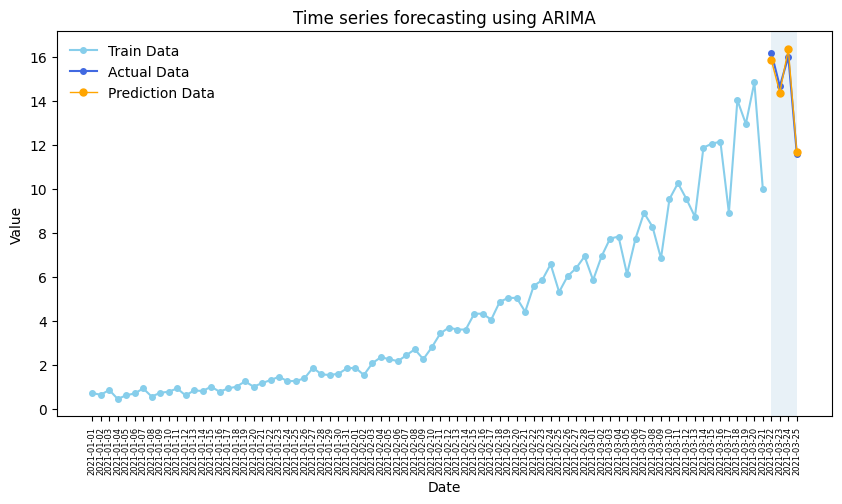
# In our case, we use the previous 80 days to train the model and predict the last 4 days. 
ARIMA_pred = model_fit.get_prediction(80, 83).predicted_mean # model_fit.forecast(steps=4)

ARIMA_pred

80    15.856387
81    14.382198
82    16.369116
83    11.681353
Name: predicted_mean, dtype: float64

# Plotting
plt.figure(figsize=(10, 5))
plt.plot(df_data.date[:-4].values, train_data.values, color='skyblue', lw=1.5, marker='o', markersize=4, label='Train Data')
plt.plot(df_data.date[-4:].values, test_data.values, color='royalblue', lw=1.5, marker='o',markersize=4,label='Actual Data')
plt.plot(df_data.date[-4:].values, ARIMA_pred.values, color='orange',lw=1, marker='o', markersize=5, label='Prediction Data')

# Adding labels and title
plt.xlabel('Date')
plt.ylabel('Value')
plt.title('Time series forecasting using ARIMA')
plt.legend(frameon=False)
plt.axvspan(80,83, alpha=0.1)
plt.xticks(fontsize=6, rotation=90)  # Adjust fontsize and rotation angle
plt.show()

Some metrics: MAPE, MSE

from sklearn.metrics import mean_squared_error, mean_absolute_percentage_error

# ARIMA Vs Naive(use fromer values represent the predicted values)
naive_pred = df_data.data[76:80]

# Calculate Mean Squared Error (MSE)
mse_a = mean_squared_error(test_data, ARIMA_pred)
mse_n = mean_squared_error(test_data, naive_pred)
print(f"ARIMA Mean Squared Error (MSE): {mse_a}", f"Naive Mean Squared Error (MSE): {mse_n}")

# Calculate Mean Absolute Percentage Error (MAPE)
mape_a = mean_absolute_percentage_error(test_data, ARIMA_pred)
mape_n = mean_absolute_percentage_error(test_data, naive_pred)
print(f"ARIMA Mean Absolute Percentage Error (MAPE): {mape_a}", f" Naive Mean Absolute Percentage Error (MAPE): {mape_n}")

ARIMA Mean Squared Error (MSE): 0.08196834766291569 Naive Mean Squared Error (MSE): 2.8957499999999987
ARIMA Mean Absolute Percentage Error (MAPE): 0.017191860828344573  Naive Mean Absolute Percentage Error (MAPE): 0.11561658552433654

4.4 SARIMA(\(p,d,q\))(\(P,D,Q\))\(m\)

Seasonal autoregressive integrated moving average (SARIMA) model adds seasonal parameters to the ARIMA(p,d,q) model.

It is denoted as SARIMA(\(p,d,q\))(\(P,D,Q\))\(m\), where

• \(P\) is the order of the seasonal AR(\(P\)) process;

• \(D\) is the seasonal order of integration;

• \(Q\) is the order of the seasonal MA(\(Q\))process;

• \(m\) is the frequency or the number of observations per seasonal cycle.

Note that a SARIMA(\(p,d,q\))(\(0,0,0\))\(m\) model is equivalent to an ARIMA(\(p,d,q\)) model.

4.4.1 What is frequencey \(m\)?

Appropriate frequency \(m\) depending on the data:

Data collection	Frequencey \(m\) (observation unit/level)
Annual	1
Quarterly	4
Monthly	12
Weekly	52
Daily	365
Hourly	8760

Please download the sample data here.

# use the air passengers data for analysis
df_ap = pd.read_csv('air-passengers.csv', index_col=0)

df_ap.head()

	Passengers
Month
1949-01	112
1949-02	118
1949-03	132
1949-04	129
1949-05	121

# set index to datatime type
df_ap.index = pd.to_datetime(df_ap.index)

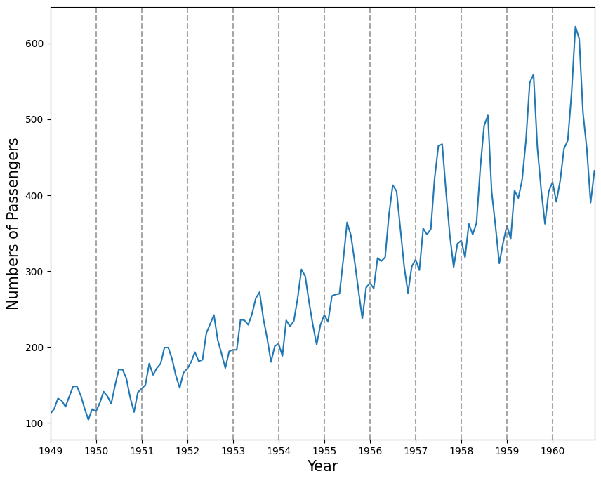
Plotting the time series datacan help to observe periodic patterns (frequencey).

# Plot the time series
df_ap.plot(figsize=(10, 8), legend=False)

# Add vertical lines for each year
years = pd.to_datetime(df_ap.index.year.unique().values, format='%Y')
for year in years:
    plt.axvline(x=year, color='grey', linestyle='--', alpha=0.7)

plt.xticks(years, labels=df_ap.index.year.unique().values)
plt.xlabel('Year', fontsize=15)
plt.ylabel('Numbers of Passengers', fontsize=15)
plt.show()

Another way of identifying seasonal patterns is using time series decomposition.

Note: In a time series without a seasonal pattern, the decomposition process will show the seasonal component as a flat horizontal line at 0.

## decomposition of time series
from statsmodels.tsa.seasonal import STL
decomposition = STL(df_ap['Passengers'], period=12).fit()

fig, (ax1, ax2, ax3, ax4) = plt.subplots(nrows=4, ncols=1, sharex=True, figsize=(8,6))
ax1.plot(decomposition.observed)
ax1.set_ylabel('Observed')
ax2.plot(decomposition.trend)
ax2.set_ylabel('Trend')
ax3.plot(decomposition.seasonal)
ax3.set_ylabel('Seasonal')
ax4.plot(decomposition.resid)
ax4.set_ylabel('Residuals')
fig.autofmt_xdate()
plt.tight_layout()

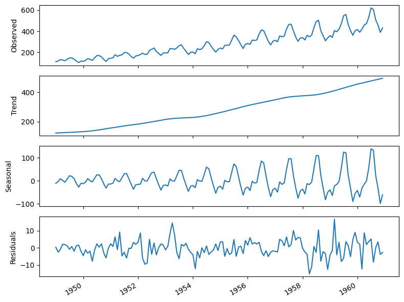
Interpretation:

• The summer months (July and August) usually have the highest numbers of air passengers in one year;

• If we are to forecast the month of July in 1961, the information coming from the month of July in prior years is likely going to be useful, since we can intuitively expect the number of air passengers to be at its highest point in the month of July 1961;

• The parameters \(P, D, Q,\) and \(m\) allow us to capture that information from the previous seasonal cycle and help us forecast our time series.

4.4.2 Forecasting using a SRIMA model

# The result of ADF test show this time series is non-stationary
ad_fuller_result = adfuller(df_ap['Passengers'])
print(f'ADF Statistic: {ad_fuller_result[0]}')
print(f'p-value: {ad_fuller_result[1]}')

ADF Statistic: 0.8153688792060446
p-value: 0.9918802434376409

# The hyperparameter tuning of SARIMA
from typing import Union
from statsmodels.tsa.statespace.sarimax import SARIMAX

def optimize_SARIMA(endog: Union[pd.Series, list], order_list:list, m:int):
    results = []
    for order in order_list:
        try:
            model = SARIMAX(endog, 
                            order=(order[0], order[1], order[2]), 
                            seasonal_order=(order[3], order[4], order[5], m),
                            simple_differencing=False).fit(disp=False)
            aic = model.aic
            results.append([order[0:3], order[3:], aic])
        except Exception as e:
            # Print or log the exception if needed
            print(f"Error encountered for order {order}: {str(e)}")
            continue

    # Convert results to DataFrame and sort by AIC
    result_df = pd.DataFrame(results, columns=['(p,d,q)','(P,D,Q)', 'AIC'])
    result_df = result_df.sort_values(by='AIC', ascending=True).reset_index(drop=True)
    return result_df

# Set the ranges of parameters
from itertools import product
ps = range(0, 3, 1) 
ds = range(1, 3, 1)
qs = range(0, 3, 1)   

Ps = range(0, 3, 1)
Ds = range(1, 3, 1)
Qs = range(0, 3, 1)
m = 12

SARIMA_order_list = list(product(ps,ds,qs,Ps,Ds,Qs))
print(len(SARIMA_order_list), 'sets of parameters')

324 sets of parameters

# Training and testing set
train = df_ap['Passengers'][:-12]
test = df_ap['Passengers'][-12:]

%%time

import warnings
warnings.filterwarnings('ignore')

SARIMA_result_df = optimize_SARIMA(train, SARIMA_order_list, 12)

CPU times: user 3min 35s, sys: 1min 42s, total: 5min 17s
Wall time: 3min 46s

# The result df
SARIMA_result_df

	(p,d,q)	(P,D,Q)	AIC
0	(1, 1, 0)	(0, 2, 2)	821.076627
1	(0, 1, 1)	(0, 2, 2)	821.837043
2	(1, 1, 0)	(1, 2, 1)	821.936210
3	(1, 1, 0)	(1, 2, 2)	822.749933
4	(0, 1, 1)	(1, 2, 1)	823.011902
...	...	...	...
319	(0, 2, 0)	(2, 1, 0)	1004.515070
320	(0, 2, 0)	(0, 1, 0)	1004.691880
321	(0, 2, 0)	(2, 1, 2)	1005.651588
322	(0, 2, 0)	(2, 1, 1)	1006.262253
323	(0, 2, 0)	(1, 1, 2)	1006.296666

324 rows × 3 columns

# Selecting the optimised parameters for SARIMA
SARIMA_model = SARIMAX(train, order=(1,1,0), seasonal_order=(0,2,2,12), simple_differencing=False)
SARIMA_model_fit = SARIMA_model.fit(disp=False)

# The residual analysis for optimised SARIMA, see the interpretation listed in the last section.
SARIMA_model_fit.plot_diagnostics(figsize=(10,8))
plt.show()

# Ljung-Box test
from statsmodels.stats.diagnostic import acorr_ljungbox
residuals = SARIMA_model_fit.resid
acorr_ljungbox(residuals, np.arange(1, 11, 1))

	lb_stat	lb_pvalue
1	0.085536	0.769931
2	1.102154	0.576329
3	1.107583	0.775244
4	1.115446	0.891814
5	1.356057	0.929059
6	1.430651	0.963967
7	1.933380	0.963435
8	2.159701	0.975720
9	2.179859	0.988293
10	4.478778	0.923175

# Based on the results from residual analysis and Ljung-Box test, 
# we can use this model to forecast the next 12 months
SARIMA_pred = SARIMA_model_fit.forecast(steps=12)
SARIMA_pred

1960-01-01    420.748114
1960-02-01    399.592088
1960-03-01    463.924725
1960-04-01    452.693368
1960-05-01    476.834224
1960-06-01    541.861652
1960-07-01    617.871434
1960-08-01    629.561211
1960-09-01    523.688112
1960-10-01    464.829748
1960-11-01    414.556494
1960-12-01    456.165585
Freq: MS, Name: predicted_mean, dtype: float64

Use ARIMA to predict the last 12 months and compare to SARIMA

# set the ranges of parameters, here we also use the SARIMA-optimised function 
 
ps = range(0, 10, 1) 
ds = range(1, 5, 1)
qs = range(0, 10, 1)   

# Here, we set P,D,Q,m as 0, then build an ARIMA (a SARIMA(p,d,q)(0,0,0)m model is equivalent to an ARIMA(p,d,q) model.)
Ps = range(0, 1, 1) 
Ds = range(0, 1, 1)
Qs = range(0, 1, 1)
m = 0

ARIMA_order_list = list(product(ps,ds,qs,Ps,Ds,Qs))
print(len(ARIMA_order_list), 'sets of parameters')

400 sets of parameters

%%time

import warnings
warnings.filterwarnings('ignore')
ARIMA_result_df = optimize_SARIMA(train, ARIMA_order_list, 12)
ARIMA_result_df

CPU times: user 1min 21s, sys: 2min 22s, total: 3min 44s
Wall time: 1min 39s

	(p,d,q)	(P,D,Q)	AIC
0	(9, 1, 9)	(0, 0, 0)	1133.935851
1	(8, 2, 8)	(0, 0, 0)	1135.116690
2	(8, 1, 8)	(0, 0, 0)	1137.434579
3	(8, 1, 9)	(0, 0, 0)	1139.745570
4	(9, 2, 8)	(0, 0, 0)	1142.817741
...	...	...	...
395	(0, 3, 0)	(0, 0, 0)	1413.932027
396	(3, 4, 0)	(0, 0, 0)	1415.764808
397	(2, 4, 0)	(0, 0, 0)	1422.180152
398	(1, 4, 0)	(0, 0, 0)	1475.515080
399	(0, 4, 0)	(0, 0, 0)	1544.442955

400 rows × 3 columns

# Selecting the optimised parameters for ARIMA
ARIMA_model = SARIMAX(train, order=(8,2,8), seasonal_order=(0,0,0,0), simple_differencing=False)
ARIMA_model_fit = ARIMA_model.fit(disp=False)
# Forecasting next 12 months
ARIMA_pred = ARIMA_model_fit.forecast(steps=12)
ARIMA_pred

1960-01-01    408.670683
1960-02-01    363.259163
1960-03-01    383.244324
1960-04-01    406.585123
1960-05-01    484.484319
1960-06-01    541.506475
1960-07-01    564.414142
1960-08-01    533.462905
1960-09-01    487.088071
1960-10-01    484.185290
1960-11-01    427.291665
1960-12-01    423.433546
Freq: MS, Name: predicted_mean, dtype: float64

Note: Run the residual for ARIMA and generate the interpretation

Comparing the performace for SARIMA and ARIMA

df_test = pd.DataFrame(test)
df_test['ARIMA_pred'] = ARIMA_pred.values
df_test['SARIMA_pred'] = SARIMA_pred.values

df_test

	Passengers	ARIMA_pred	SARIMA_pred
Month
1960-01-01	417	408.670683	420.748114
1960-02-01	391	363.259163	399.592088
1960-03-01	419	383.244324	463.924725
1960-04-01	461	406.585123	452.693368
1960-05-01	472	484.484319	476.834224
1960-06-01	535	541.506475	541.861652
1960-07-01	622	564.414142	617.871434
1960-08-01	606	533.462905	629.561211
1960-09-01	508	487.088071	523.688112
1960-10-01	461	484.185290	464.829748
1960-11-01	390	427.291665	414.556494
1960-12-01	432	423.433546	456.165585

## Plot the prediction plot
fig, ax = plt.subplots(figsize=(10,8))
ax.plot(df_ap['Passengers'], 'skyblue')
ax.plot(df_test['Passengers'], 'k-', label='observed')
ax.plot(df_test['ARIMA_pred'], 'b--', label='ARIMA(8,2,8)')
ax.plot(df_test['SARIMA_pred'], 'g--', label='SARIMA(1,1,0)(0,2,2,12)')
ax.set_xlabel('Month')
ax.set_ylabel('Number of Passengers')
ax.axvspan('1960-01', '1960-12', color='#808080', alpha=0.2)
ax.legend(loc=2, fontsize=15, frameon=False)
ax.set_xlim(pd.to_datetime("1959-01-01"), pd.to_datetime("1960-12-01")) 
ax.set_ylim(280, 650)
plt.xticks(fontsize=12, rotation=0)  # Adjust font size and rotation angle
plt.tight_layout()

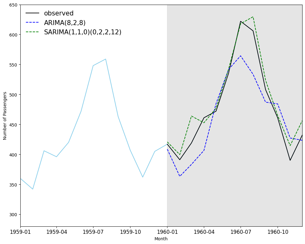
 # ARIMA Vs SARIMA 
 
# Calculate Mean Squared Error (MSE)
mse_arima = mean_squared_error(test, ARIMA_pred)
mse_sarima = mean_squared_error(test, SARIMA_pred)
print(f"ARIMA MSE : {mse_arima}", 
      f"SARIMA MSE : {mse_sarima}")

# Calculate Mean Absolute Percentage Error (MAPE)
mape_arima = mean_absolute_percentage_error(test, ARIMA_pred)
mape_sarima = mean_absolute_percentage_error(test, SARIMA_pred)
print(f"ARIMA MAPE: {mape_arima}",
      f"SARIMA MAPE: {mape_sarima}")

ARIMA MSE : 1357.7709262001347 SARIMA MSE : 355.45931874052184
ARIMA MAPE: 0.06267455525110724 SARIMA MAPE: 0.03190661271178543

4.5 Machine learning models (XGBoost)

# We use the air passenger data as an example
df_ap = pd.read_csv('air-passengers.csv', index_col=0)
# set index to datatime type
df_ap.index = pd.to_datetime(df_ap.index)

df_ap

	Passengers
Month
1949-01-01	112
1949-02-01	118
1949-03-01	132
1949-04-01	129
1949-05-01	121
...	...
1960-08-01	606
1960-09-01	508
1960-10-01	461
1960-11-01	390
1960-12-01	432

144 rows × 1 columns

# create an month and generate basic features
df_ap['Month'] = pd.to_datetime(df_ap.index)
df_ap['month'] = df_ap['Month'].dt.month
df_ap['quarter'] = df_ap['Month'].dt.quarter
df_ap['year'] = df_ap['Month'].dt.year
df_ap.drop(columns=['Month'])

	Passengers	month	quarter	year
Month
1949-01-01	112	1	1	1949
1949-02-01	118	2	1	1949
1949-03-01	132	3	1	1949
1949-04-01	129	4	2	1949
1949-05-01	121	5	2	1949
...	...	...	...	...
1960-08-01	606	8	3	1960
1960-09-01	508	9	3	1960
1960-10-01	461	10	4	1960
1960-11-01	390	11	4	1960
1960-12-01	432	12	4	1960

144 rows × 4 columns

# create lagged features (shift to right)
for lag in range(1,25):
    df_ap[f'lag_{lag}'] = df_ap['Passengers'].shift(lag).values

df_ap

	Passengers	Month	month	quarter	year	lag_1	lag_2	lag_3	lag_4	lag_5	...	lag_15	lag_16	lag_17	lag_18	lag_19	lag_20	lag_21	lag_22	lag_23	lag_24
Month
1949-01-01	112	1949-01-01	1	1	1949	NaN	NaN	NaN	NaN	NaN	...	NaN	NaN	NaN	NaN	NaN	NaN	NaN	NaN	NaN	NaN
1949-02-01	118	1949-02-01	2	1	1949	112.0	NaN	NaN	NaN	NaN	...	NaN	NaN	NaN	NaN	NaN	NaN	NaN	NaN	NaN	NaN
1949-03-01	132	1949-03-01	3	1	1949	118.0	112.0	NaN	NaN	NaN	...	NaN	NaN	NaN	NaN	NaN	NaN	NaN	NaN	NaN	NaN
1949-04-01	129	1949-04-01	4	2	1949	132.0	118.0	112.0	NaN	NaN	...	NaN	NaN	NaN	NaN	NaN	NaN	NaN	NaN	NaN	NaN
1949-05-01	121	1949-05-01	5	2	1949	129.0	132.0	118.0	112.0	NaN	...	NaN	NaN	NaN	NaN	NaN	NaN	NaN	NaN	NaN	NaN
...	...	...	...	...	...	...	...	...	...	...	...	...	...	...	...	...	...	...	...	...	...
1960-08-01	606	1960-08-01	8	3	1960	622.0	535.0	472.0	461.0	419.0	...	420.0	396.0	406.0	342.0	360.0	337.0	310.0	359.0	404.0	505.0
1960-09-01	508	1960-09-01	9	3	1960	606.0	622.0	535.0	472.0	461.0	...	472.0	420.0	396.0	406.0	342.0	360.0	337.0	310.0	359.0	404.0
1960-10-01	461	1960-10-01	10	4	1960	508.0	606.0	622.0	535.0	472.0	...	548.0	472.0	420.0	396.0	406.0	342.0	360.0	337.0	310.0	359.0
1960-11-01	390	1960-11-01	11	4	1960	461.0	508.0	606.0	622.0	535.0	...	559.0	548.0	472.0	420.0	396.0	406.0	342.0	360.0	337.0	310.0
1960-12-01	432	1960-12-01	12	4	1960	390.0	461.0	508.0	606.0	622.0	...	463.0	559.0	548.0	472.0	420.0	396.0	406.0	342.0	360.0	337.0

144 rows × 29 columns

# Training and testing data set

training_data = df_ap.query('Month < "1960-01-01"')
print(training_data.shape)

testing_data = df_ap.query('Month >= "1960-01-01"')
print(testing_data.shape)

X_train = training_data[['month', 'quarter', 'year']]
y_train = training_data['Passengers']
 
X_test = testing_data[['month', 'quarter', 'year']]
y_test = testing_data['Passengers']

(132, 29)
(12, 29)

%%time
from xgboost import XGBRegressor
from sklearn.model_selection import TimeSeriesSplit, GridSearchCV
 
# XGBoost
cv_split = TimeSeriesSplit(n_splits=4, test_size=30)
model = XGBRegressor()
parameters = {
    "max_depth": [3, 5, 10],
    "learning_rate": [0.01, 0.05, 0.1, 0.3],
    "n_estimators": [50, 100, 300, 500],
    "colsample_bytree": [0.3, 0.5, 0.7, 0.9]
 }
 
 
grid_search = GridSearchCV(estimator=model, cv=cv_split, param_grid=parameters, scoring='neg_mean_squared_error')
grid_search.fit(X_train, y_train)

CPU times: user 2min 6s, sys: 14min 16s, total: 16min 22s
Wall time: 3min 46s

GridSearchCV(cv=TimeSeriesSplit(gap=0, max_train_size=None, n_splits=4, test_size=30),
             estimator=XGBRegressor(base_score=None, booster=None,
                                    callbacks=None, colsample_bylevel=None,
                                    colsample_bynode=None,
                                    colsample_bytree=None, device=None,
                                    early_stopping_rounds=None,
                                    enable_categorical=False, eval_metric=None,
                                    feature_types=None, gamma=None,
                                    grow_policy=None, impor...
                                    max_depth=None, max_leaves=None,
                                    min_child_weight=None, missing=nan,
                                    monotone_constraints=None,
                                    multi_strategy=None, n_estimators=None,
                                    n_jobs=None, num_parallel_tree=None,
                                    random_state=None, ...),
             param_grid={'colsample_bytree': [0.3, 0.5, 0.7, 0.9],
                         'learning_rate': [0.01, 0.05, 0.1, 0.3],
                         'max_depth': [3, 5, 10],
                         'n_estimators': [50, 100, 300, 500]},
             scoring='neg_mean_squared_error')

In a Jupyter environment, please rerun this cell to show the HTML representation or trust the notebook.
On GitHub, the HTML representation is unable to render, please try loading this page with nbviewer.org.

# best params for xgboost
print(grid_search.best_params_)

{'colsample_bytree': 0.7, 'learning_rate': 0.3, 'max_depth': 3, 'n_estimators': 500}

# optimised xgboost
best_model = grid_search.best_estimator_

from sklearn.metrics import mean_absolute_error, mean_absolute_percentage_error, mean_squared_error
 
def evaluate_model(y_test, prediction):
      # print(f"MAE: {mean_absolute_error(y_test, prediction)}")
      print(f"MSE: {mean_squared_error(y_test, prediction)}")
      print(f"MAPE: {mean_absolute_percentage_error(y_test, prediction)}")

# Evaluating GridSearch results
XGBOOST_pred = best_model.predict(X_test)
# plot_predictions(testing_dates, y_test, prediction)
evaluate_model(y_test, XGBOOST_pred)

MSE: 2563.708906709915
MAPE: 0.09997636162436208

Further exploration:

• Why XGBoost performace is worse than SARIMA on this data?

• Any techniques can be used to improve the XGBoost (rolling forecasting, more featuring engineering)?

• Deep learning model (RNN, LSTM, CNN)?

• Bigger Data?