5 Network analysis#
import networkx as nx
import pandas as pd
import matplotlib.pyplot as plt
5.1 Basic concepts of network#
A network is frequently used interchangeably with a graph, but it typically highlights real-world applications and is commonly associated with social relationships (social networks), and built environments (road networks).
A graph (\(G\)) is a mathematical structure used to model pairwise relations between objects. It consists of a set of vertices (nodes) and a set of edges (links) that connect pairs of vertices.
Graph Type
Graph Type |
Description |
NetworkX Class |
|---|---|---|
Undirected Graph |
A graph where edges have no direction. |
Graph |
Directed Graph |
A graph where edges have a direction, indicated by an arrow. |
DiGraph |
Multi-(undirected) Graph |
An undirected graph with parallel edges. |
MultiGraph |
Multi-directed Graph |
A directed graph with parallel edges. |
MultiDiGraph |
Note: All types of graphs can have self-loops.
5.2 Measurements for nodes and edges#
# Create an empty undirected graph
G = nx.Graph()
# Add edge with weight
G.add_edge(1, 2, weight=30)
G.add_edge(1, 3, weight=5)
G.add_edge(2, 3, weight=22)
G.add_edge(2, 4, weight=2)
G.add_edge(3, 4, weight=37)
# Print edge infos
print(G.edges(data=True))
[(1, 2, {'weight': 30}), (1, 3, {'weight': 5}), (2, 3, {'weight': 22}), (2, 4, {'weight': 2}), (3, 4, {'weight': 37})]
# Print node infos, the {} represents the node attributes for each node, e.g, you can input {'attribute_name': 'value'}
print(G.nodes(data=True))
[(1, {}), (2, {}), (3, {}), (4, {})]
# Print weight info
weights = nx.get_edge_attributes(G, 'weight')
weights
{(1, 2): 30, (1, 3): 5, (2, 3): 22, (2, 4): 2, (3, 4): 37}
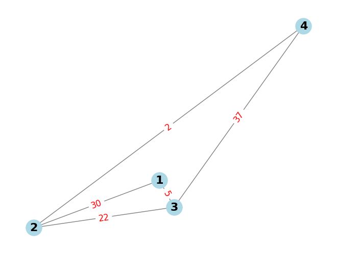
# Network draw
pos = nx.random_layout(G)

nx.draw(G, pos, with_labels=True, node_color='lightblue', edge_color='gray', node_size=500, font_size=16, font_weight='bold')

# Draw edge labels (weights)
edge_labels = nx.get_edge_attributes(G, 'weight')
nx.draw_networkx_edge_labels(G, pos, edge_labels=edge_labels, font_color='red', font_size=12)
{(1, 2): Text(0.5561991977914811, 0.12568247125450527, '30'),
 (1, 3): Text(0.7006559471724646, 0.1625788871207906, '5'),
 (2, 3): Text(0.5711164605781995, 0.0773496395248637, '22'),
 (2, 4): Text(0.7041137349515878, 0.4039085552972916, '2'),
 (3, 4): Text(0.8485686428703795, 0.4408032318889426, '37')}
5.2.1 Degree centrality of nodes#
The degree centrality values are normalized by dividing by the maximum possible degree in a simple graph n-1 where n is the number of nodes in \(G\).
# networkx
nx.degree_centrality(G)
{1: 0.6666666666666666, 2: 1.0, 3: 1.0, 4: 0.6666666666666666}
5.2.2 Closeness centrality of nodes#
Closeness centrality of a node \(u\) is the reciprocal of the average shortest path distance to \(u\) over all \(n-1\) reachable nodes.
\(G =(U,V)\).
\(C(v) = \frac{n-1}{\sum_{v =1}^{n-1} d(v, u)}\)
where \(d(v, u)\) is the shortest-path distance between v and u, and n-1 is the number of nodes reachable from \(u\).
Shortest path and distance
1->2 : 1,3,2 (5+22 = 27)
1->3: 1,3 (5)
1->4: 1,3,2,4 (5+22+2=29)
2->3: 2,3 (22)
2->4: 2,4 (2)
3->4: 3,2,4 (22+2=24)
# use networkx to get shoreat path distance
nx.shortest_path_length(G, 1, 2, weight='weight')
27
nx.shortest_path_length(G, 1, 3, weight='weight')
5
nx.shortest_path_length(G, 1, 4, weight='weight')
29
nx.shortest_path_length(G, 2, 3, weight='weight')
22
nx.shortest_path_length(G, 2, 4, weight='weight')
2
nx.shortest_path_length(G, 3, 4, weight='weight')
24
# cc of node 1
(4-1) / (27 + 5 + 29)
0.04918032786885246
# cc of node 2
(4-1) / (27 + 22 + 2)
0.058823529411764705
# cc of node3
(4-1) / (5 + 22 + 24)
0.058823529411764705
# cc of node 4
(4-1) / (29 + 2 + 24)
0.05454545454545454
# use nx to get cc
nx.closeness_centrality(G, distance='weight')
{1: 0.04918032786885246,
 2: 0.058823529411764705,
 3: 0.058823529411764705,
 4: 0.05454545454545454}
5.2.3 Betweenness centrality of nodes#
Betweenness centrality of a node \(v\) is the sum of the fraction of all-pairs shortest paths that pass through \(v\).
\(C_B(v) = \sum_{s,t \in V} \frac{\sigma({s,t |v })}{\sigma({s, t})}\)
where \(V\) is the set of nodes,
\(\sigma({s, t})\) is the number of shortest paths,
\(\sigma({s,t |v })\) is the number of those paths passing through some node \(v\) other than \(s,t\).
\(\text{Normalization } C_B \text{ of node} = \frac{ C_B \text{ of nodes} }{ \text{Normalization Factor} }\)
\(\text{Normalization Factor (NF) for undirected graph} = \frac{(n-1) \cdot (n-2)}{2}\)
\(n\) is the nodes numbers.
# NF
(4-1)*(4-2)/2
3.0
# Normalized betweenness centrality of node 1
0/3
0.0
# Normalized betweenness centrality of node 2
2/3
0.6666666666666666
# Normalized betweenness centrality of node 3
2/3
0.6666666666666666
# Normalized betweenness centrality of node 4
0/4
0.0
# get betweenness centrality using nx
nx.betweenness_centrality(G,  weight='weight', normalized=True)
{1: 0.0, 2: 0.6666666666666666, 3: 0.6666666666666666, 4: 0.0}
5.2.4 Betweenness centrality of edges#
Betweenness centrality of an edge \(e\) is the sum of the fraction of all-pairs shortest paths that pass through \(e\).
\(C_B(e) = \sum_{s,t \in V} \frac{\sigma({s,t |e})}{\sigma({s, t})}\)
where \(V\) is the set of nodes,
\(\sigma({s, t})\) is the number of shortest paths (\({s, t}\)),
\(\sigma({s,t |e })\) is the number of those paths passing through edge \(e\).
\(\text{Normalization } C_B \text{ of edges} = \frac{ C_B \text{ of edges} }{ \text{Normalization Factor} }\)
\(\text{Normalization Factor (NF) for undirected graph} = \frac{n(n-1)}{2}\)
n is the nodes numbers.
# Normalized betweenness centrality of edge (1,2)
0/6
0.0
# Normalized betweenness centrality of edge (1,3)
3/6
0.5
# Normalized betweenness centrality of edge (2,3)
4/6
0.6666666666666666
# Normalized betweenness centrality of edge (2,4)
3/6
0.5
# Normalized betweenness centrality of edge (3,4)
0/6
0.0
# get edge_betweenness_centrality using nx
nx.edge_betweenness_centrality(G,  weight='weight', normalized=True)
{(1, 2): 0.0,
 (1, 3): 0.5,
 (2, 3): 0.6666666666666666,
 (2, 4): 0.5,
 (3, 4): 0.0}
Note: If we create a DiGraph, are measurements still the same?
Gd = nx.DiGraph()
Gd.add_edge(1, 2, weight=30)
Gd.add_edge(1, 3, weight=5)
Gd.add_edge(2, 3, weight=22)
Gd.add_edge(2, 4, weight=2)
Gd.add_edge(3, 4, weight=37)